Visualizing LeNet-5

LeNet-5

LeNet-5 was proposed by Yann LeCun et al. in 1998 to recognize handwritten digits (MNIST). Though simple by today’s standards, it laid the foundation for modern CNNs.

The architecture of LeNet-5 consists of the following layers:

• Convolution layers
• Pooling (subsampling) layers
• Fully connected layers

It’s a perfect candidate to visualize!

First Convolution Layer (C1)

The input image is 32x32 pixels (including a 2-pixel padding on each side). This image is processed by five 5×5 convolution filters.

Here’s what’s happening:

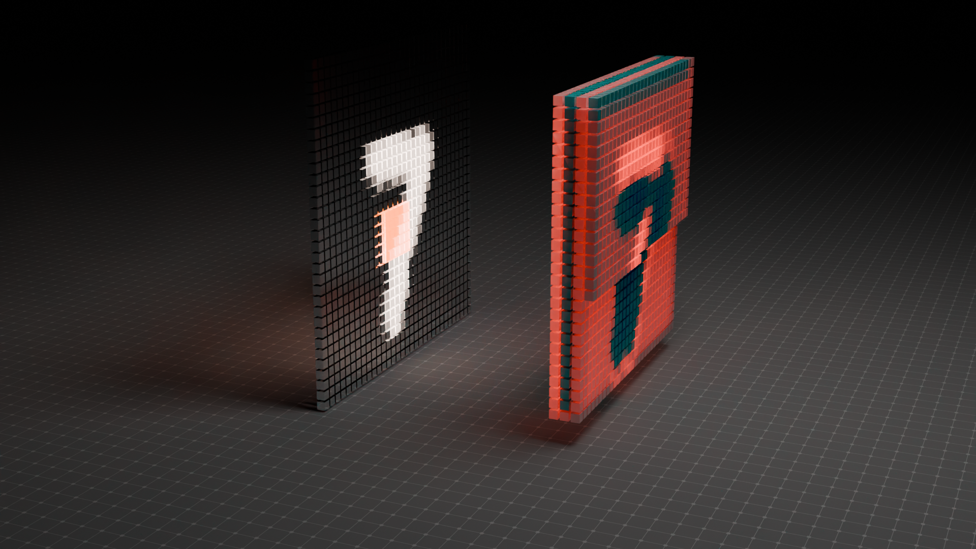
• The filter slides across the image, computing a weighted sum at each position.
• Each filter learns to detect different basic visual features (like edges or blobs).
• The result is a feature map of size 28x28.
• With 5 filters, the output is a stack of 5 feature maps → a depth of 5.

First Pooling Layer (S2)

After convolution, we apply subsampling (or pooling) to reduce the spatial dimensions while preserving important features.

Here’s what’s happening:

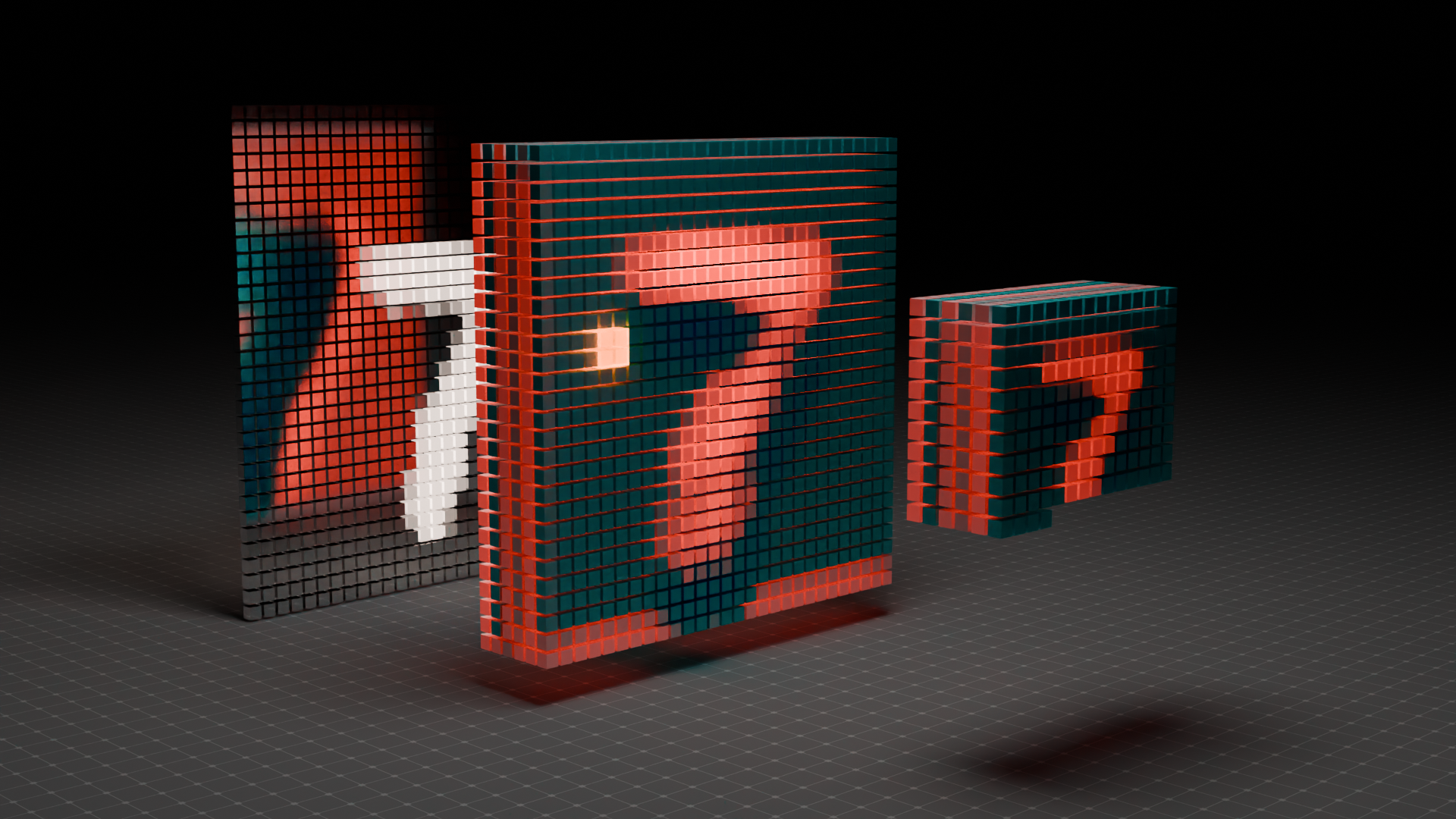
• The input to this layer is the 28×28×5 output from the previous convolution (C1).
• A 2×2 pooling filter slides over each feature map with a stride of 2.
• Each 2×2 region is reduced to a single value, typically by taking the maximum (MaxPooling).
• This operation halves the width and height while keeping the depth unchanged.
• So, the output becomes 14×14×5.

This operation helps:

• Reduce computation
• Introduce translation invariance
• Focus on the most prominent features

In the 3D visualization:

• The middle block shows the C1 output.
• The right block shows the pooled output, clearly more compact but still retaining the core structure of the input features.

Second Convolution Layer (C3)

In this stage, we apply another set of convolutions to extract deeper, more abstract features from the image. While the first convolution layer focused on basic edges and patterns, C3 begins to build hierarchical representations.

Input: 14×14×5 Output: 10 feature maps of size 10×10 → 10×10×10

Here’s what’s happening:

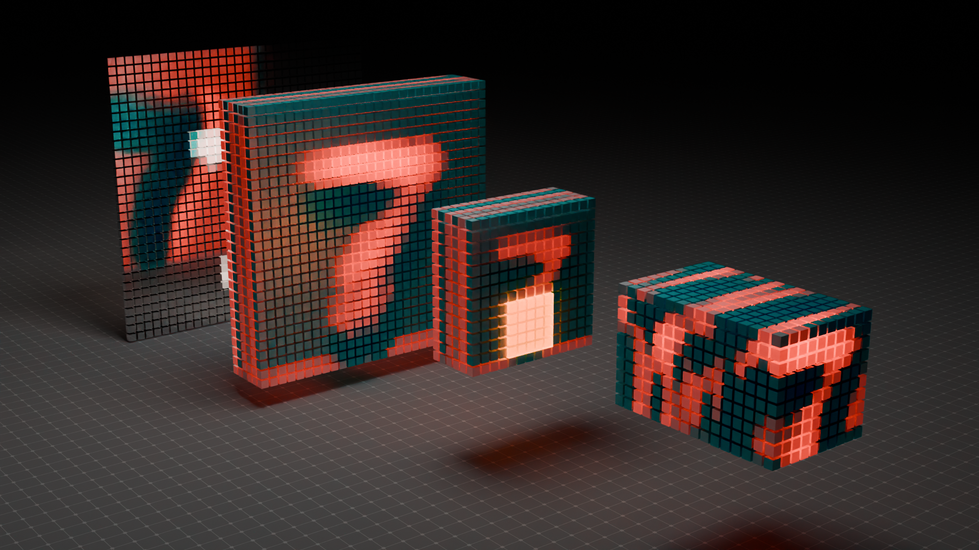
• This layer uses 5×5 filters, applied to the 5-channel input from the pooling layer (S2).
• Each output map in C3 is connected to a subset of the input maps — not all. This design was intentional in the original LeNet paper to reduce the number of parameters and encourage specialization.
• The stride is 1, and no padding is used, so the spatial dimension shrinks to 10×10.
• The output has 10 feature maps, meaning 10 filters are used in total.

In the visualization:

• The third block (from left to right) shows the C3 outputs: compact, feature-rich maps capturing meaningful shapes like digits.
• On the far right, you can see how these outputs stack into a deeper feature cube, ready for further processing.

This layer is crucial — it bridges simple visual features (like lines) with more recognizable structures (like loops, corners, or digit shapes).

Second Pooling Layer (S4)

After the second convolution layer (C3), we again apply a subsampling step to reduce spatial resolution and focus on the most prominent features.

Input to S4: 10×10×10 Output: 5×5×10

Here’s what’s happening:

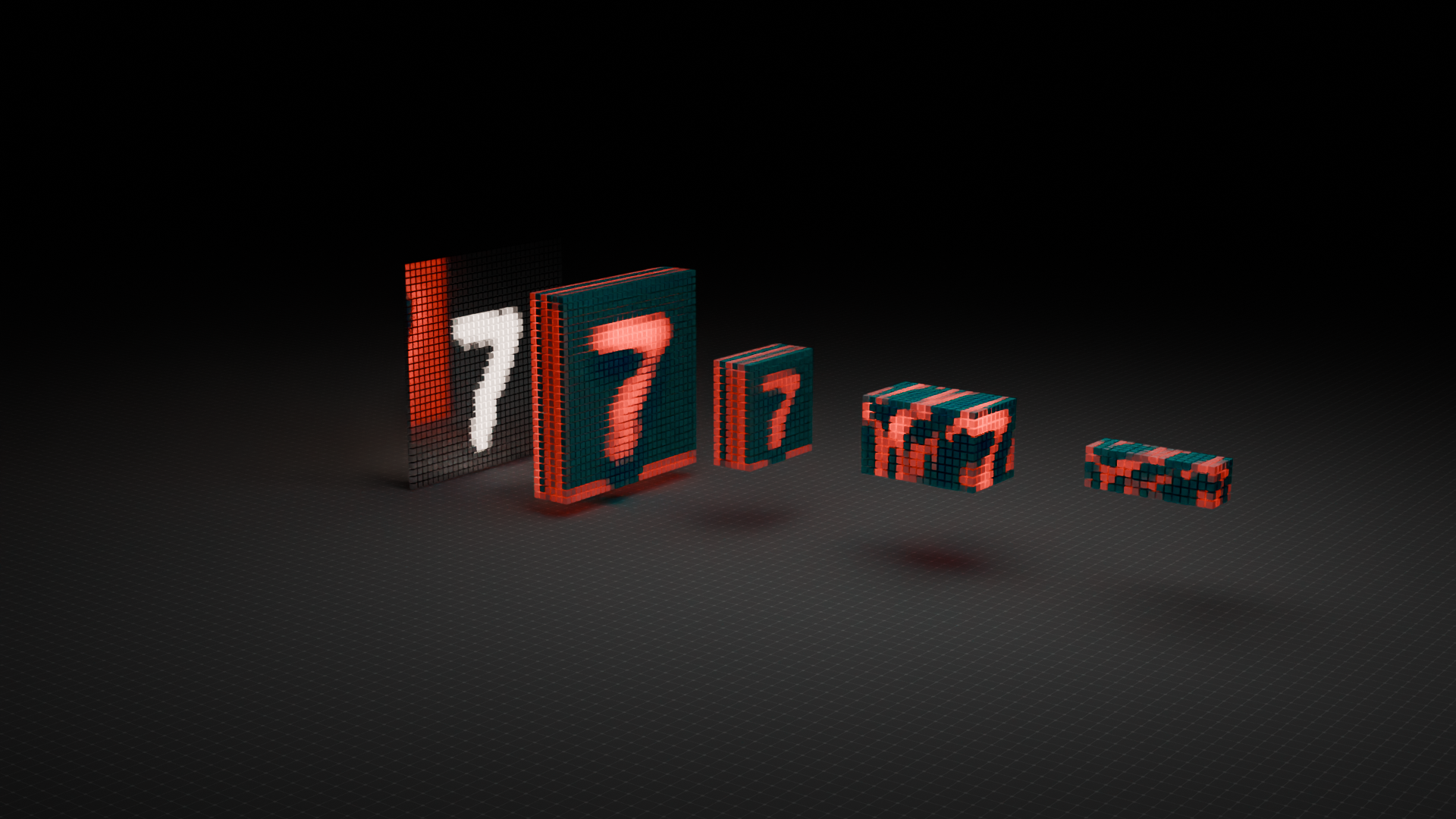
• A 2×2 pooling filter is applied with a stride of 2.
• Each 2×2 region is reduced to a single value (e.g., via MaxPooling).
• This operation shrinks the feature maps but keeps the depth (number of filters) the same.
• The resulting size is 5×5×10.

Why pooling again?

• It reduces the number of parameters before fully connected layers.
• It makes the network more robust to small translations or distortions in the input.
• It retains the essence of features while dropping redundancy.

In the visualization:

• You can see the full pipeline from left to right — from raw input to a progressively compressed and refined representation of the digit.
• The last visible block is much smaller in spatial size, but rich in learned, abstract features — ready for final classification layers.

Transition to the Fully Connected Layers (C5 → F6 → Output)

Before we enter the classic fully connected layers, LeNet-5 performs one final convolution, not a flattening step just yet.

Final Convolution Layer (C5)

At this stage, the network has compressed and abstracted the input image through multiple layers. Now we reach C5, the last convolutional layer in LeNet-5. Though it is still a convolution, it behaves like a fully connected layer in disguise.

Input to C5: 5×5×16 Output: 1×1×120 (i.e., a vector of 120 features)

Here’s what’s happening:

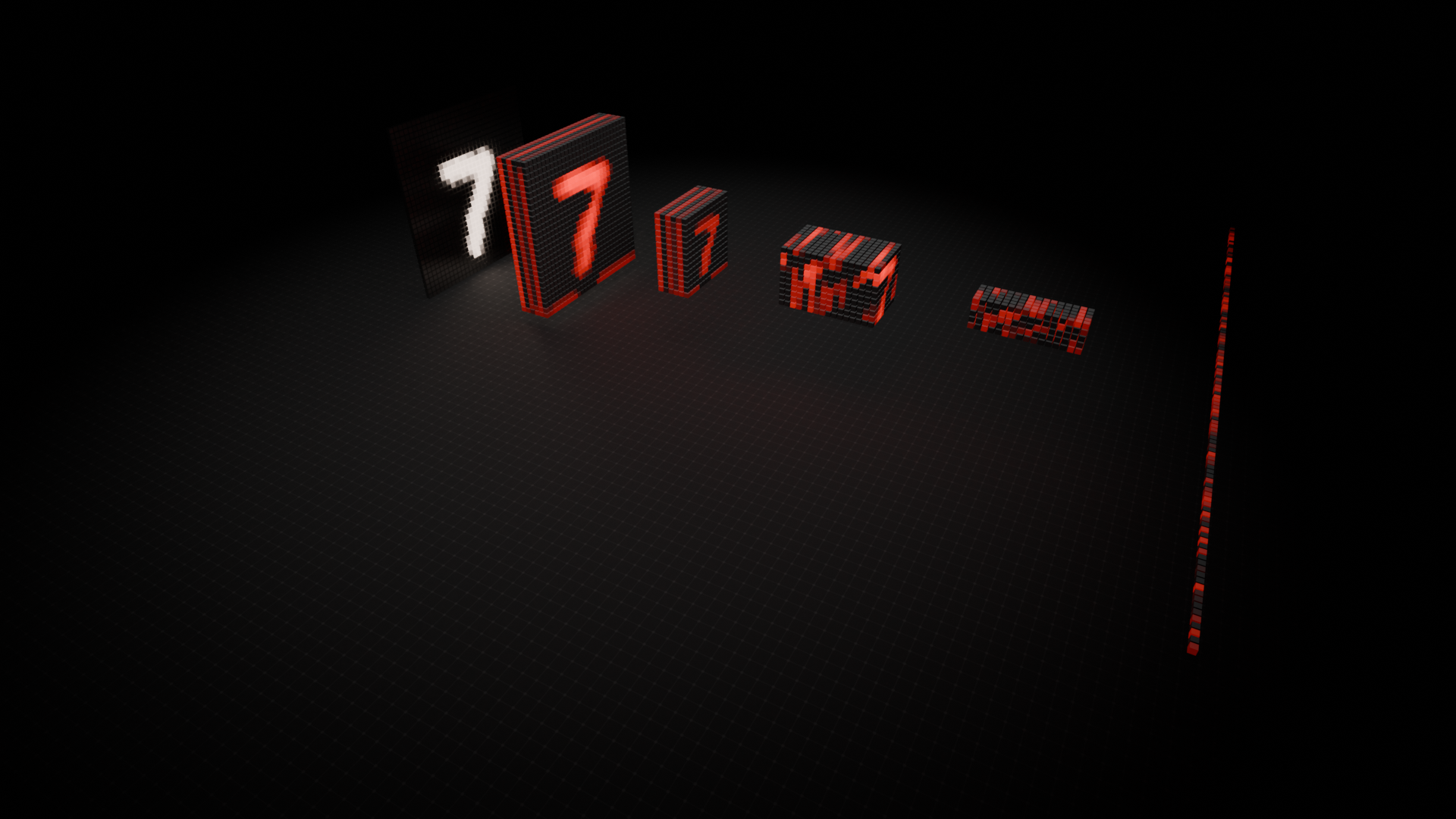
• The input has 16 feature maps, each of size 5×5.
• C5 applies 120 convolutional filters, each of size 5×5×16 (spanning the full depth).
• Since the kernel covers the entire spatial area (5×5), each filter outputs a single value.
• The result: a 120-dimensional feature vector — one scalar per filter.

Why is this important?

• It transitions the network from spatial processing (images) to feature abstraction (vectors).
• The 120 values are high-level learned features, capturing the essence of the digit shape.
• This output is ready to feed into fully connected layers for classification.

In the 3D visualization:

• On the left is the compact 5×5×16 block from the previous layer (S4).
• On the right is a vertical stack of 120 feature units — glowing elements representing abstract, distilled knowledge about the digit.
• This marks the end of the convolutional pipeline — next comes the classic neural network logic.

Fully Connected Layer (F6)

After compressing the input image through layers of convolutions and pooling, we now reach the fully connected part of LeNet-5 — where high-level reasoning happens. The first of these dense layers is called F6.

Input to F6: 120-dimensional vector (from C5) Output: 84 neurons (features)

Here’s what’s happening:

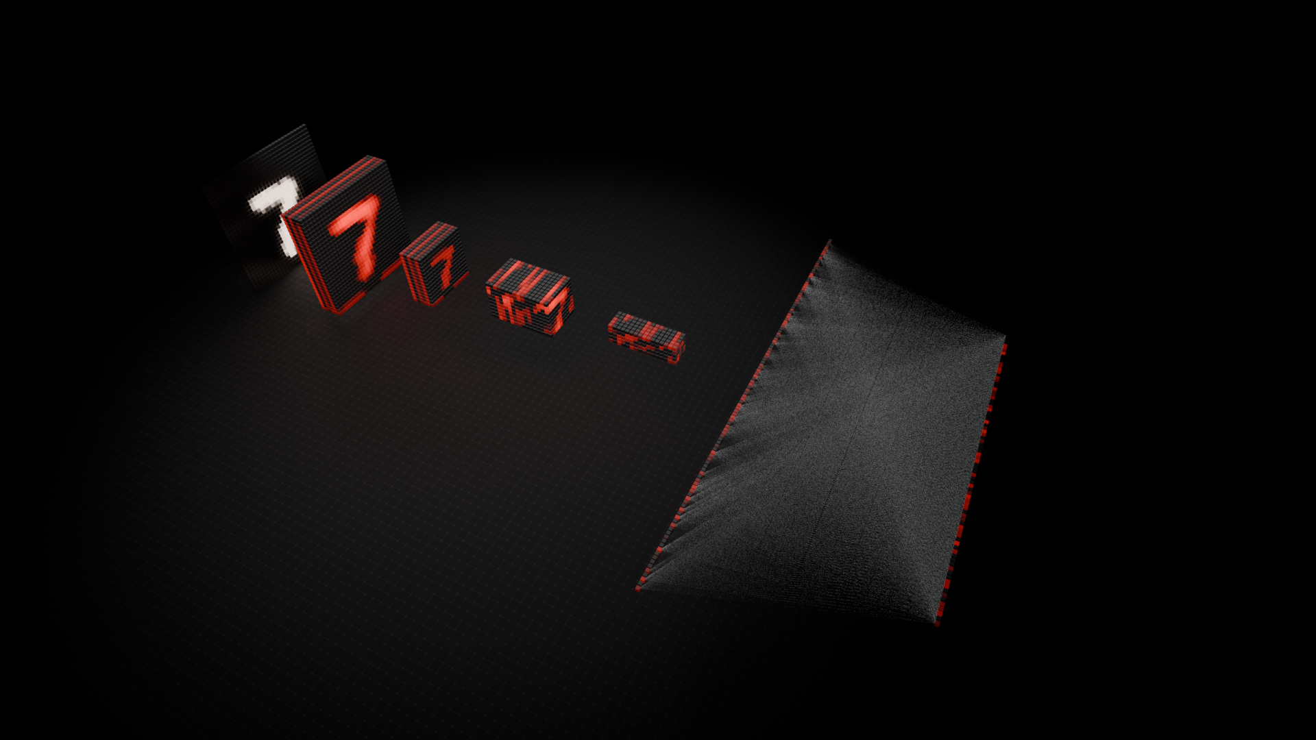
• Each of the 120 values from C5 is connected to every one of the 84 neurons in F6.
• These neurons don’t represent spatial features anymore — they encode learned patterns that are useful for digit classification.
• This dense connectivity allows the network to combine and weigh features in more abstract ways.

Why 84?

• The number is historically inspired by a biological analogy from LeCun’s original paper (linked to the number of neurons in a human visual cortex experiment).
• It’s also a sweet spot for balancing model complexity and performance on MNIST.

In the visualization:

• On the left is the output from C5: a vertical stack of 120 features.
• On the right is the 84-neuron layer, each shown as a red-lit unit in a flat rectangular grid.
• The dense mesh of connections symbolizes how every input influences every output, making this layer highly expressive.

This layer acts like a feature synthesizer, merging everything the network has learned so far and preparing for the final decision — the digit classification.

Output Layer

Everything in the LeNet-5 architecture leads to this final step: classification. The job of the output layer is simple — yet critical: decide which digit (0 through 9) the network sees in the input image.

Input to Output Layer: 84-dimensional vector (from F6) Output: 10 neurons (one for each digit class)

Here’s what’s happening:

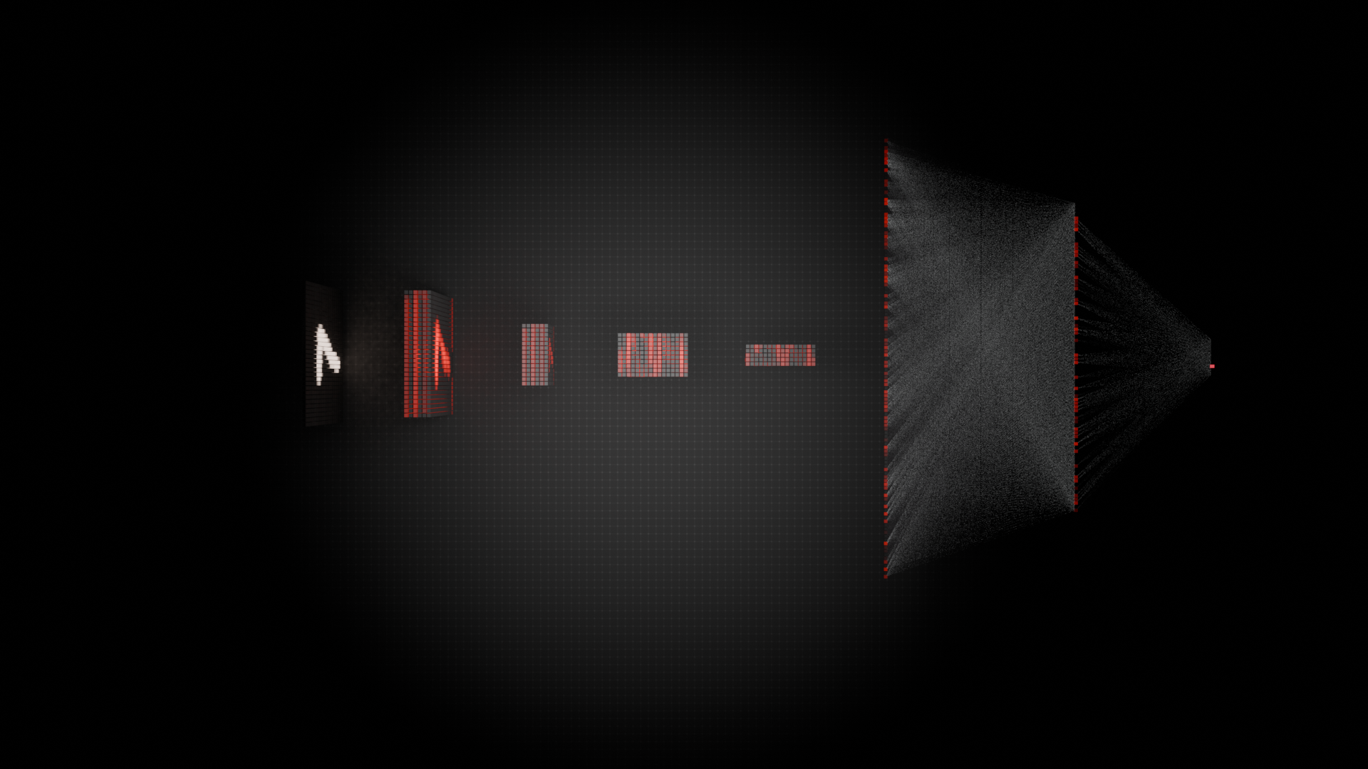
• Each of the 84 neurons from F6 is fully connected to 10 output units.
• These 10 units represent the probability scores for digits 0 through 9.
• The activation function is typically softmax, which turns raw scores into a probability distribution.
• The digit with the highest score is taken as the final prediction.

In the visualization:

• On the left, you see the dense F6 layer (84 neurons).
• On the right, a slim red vertical bar — just 10 neurons — each one a final score for a digit.
• The web of fine connections illustrates how every learned feature contributes to every output class.

This final stage brings together everything the network has learned — from edges and textures to abstract shapes — and turns it into a concrete prediction.